Figure 3

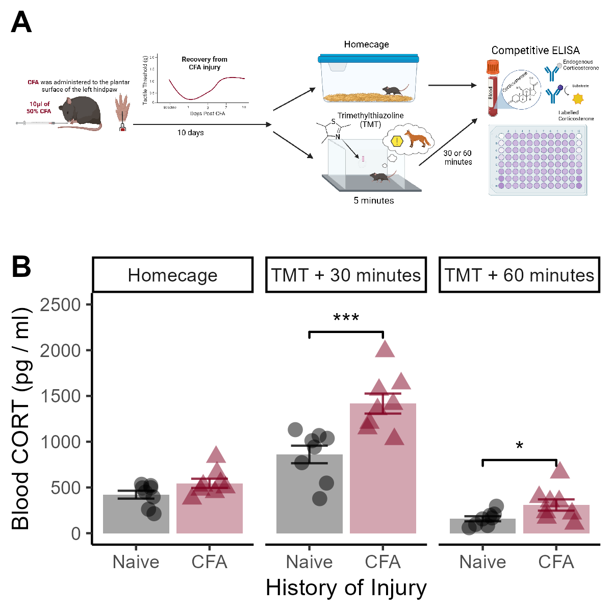
Figure 3. Mice with a history of injury have higher levels of blood corticosterone after TMT exposure. (A) Timeline of experimental procedures. Mice were injected with CFA, allowed 10 days for their injury to recover, and were then exposed to TMT for 5 minutes. Either 30 or 60 minutes after TMT, trunk blood was collected. (B) Although there is no difference in basal levels of blood corticosterone, CFA-primed mice exhibited higher levels of circulating corticosterone at both 30 and 60 minutes after TMT. Data presented as mean +/- SEM. * indicates p < 0.05, *** indicates p < 0.001.

Overall Effects of Stress and Timepoint

res <- aov(CORT ~ Stress * Pain, data = data)
summary(res)

##             Df  Sum Sq Mean Sq F value   Pr(>F)    
## Stress       2 7000783 3500391  87.218 1.11e-15 ***
## Pain         1  919426  919426  22.909 2.12e-05 ***
## Stress:Pain  2  469721  234860   5.852  0.00573 ** 
## Residuals   42 1685623   40134                     
## ---
## Signif. codes:  0 '***' 0.001 '**' 0.01 '*' 0.05 '.' 0.1 ' ' 1

Follow Ups: Effect of CFA at Each Timepoint

# Basal
a <- data %>%
  select(c("ID","Pain","Stress","CORT")) %>%
  filter(Stress == "Homecage")
  
t.test(CORT ~ Pain, data = a, var.equal = T)

## 
##  Two Sample t-test
## 
## data:  CORT by Pain
## t = -1.8737, df = 14, p-value = 0.082
## alternative hypothesis: true difference in means between group Naive and group CFA is not equal to 0
## 95 percent confidence interval:
##  -265.92402   17.94027
## sample estimates:
## mean in group Naive   mean in group CFA 
##            421.1277            545.1196

Competitive ELISA results showed no significant difference in basal corticosterone levels between groups (p = 0.08).

# 30 minutes after TMT
a <- data %>%
  select(c("ID","Pain","Stress","CORT")) %>%
  filter(Stress == "TMT_30")
  
t.test(CORT ~ Pain, data = a, var.equal = T)

## 
##  Two Sample t-test
## 
## data:  CORT by Pain
## t = -3.8218, df = 14, p-value = 0.001869
## alternative hypothesis: true difference in means between group Naive and group CFA is not equal to 0
## 95 percent confidence interval:
##  -868.3244 -244.0529
## sample estimates:
## mean in group Naive   mean in group CFA 
##            860.6665           1416.8552

# 60 minutes after TMT
a <- data %>%
  select(c("ID","Pain","Stress","CORT")) %>%
  filter(Stress == "TMT_60")
  
t.test(CORT ~ Pain, data = a, var.equal = T)

## 
##  Two Sample t-test
## 
## data:  CORT by Pain
## t = -2.2291, df = 14, p-value = 0.0427
## alternative hypothesis: true difference in means between group Naive and group CFA is not equal to 0
## 95 percent confidence interval:
##  -294.762456   -5.683044
## sample estimates:
## mean in group Naive   mean in group CFA 
##            157.9656            308.1883

However, both 30 and 60 minutes post-TMT, CFA-primed mice exhibited significantly higher circulating corticosterone levels compared to pain-naive controls (t14 = 3.82, p = 0.0018, t14 = 2.22, p = 0.043, respectively, Figure 3B).