Supplemental Figure 5

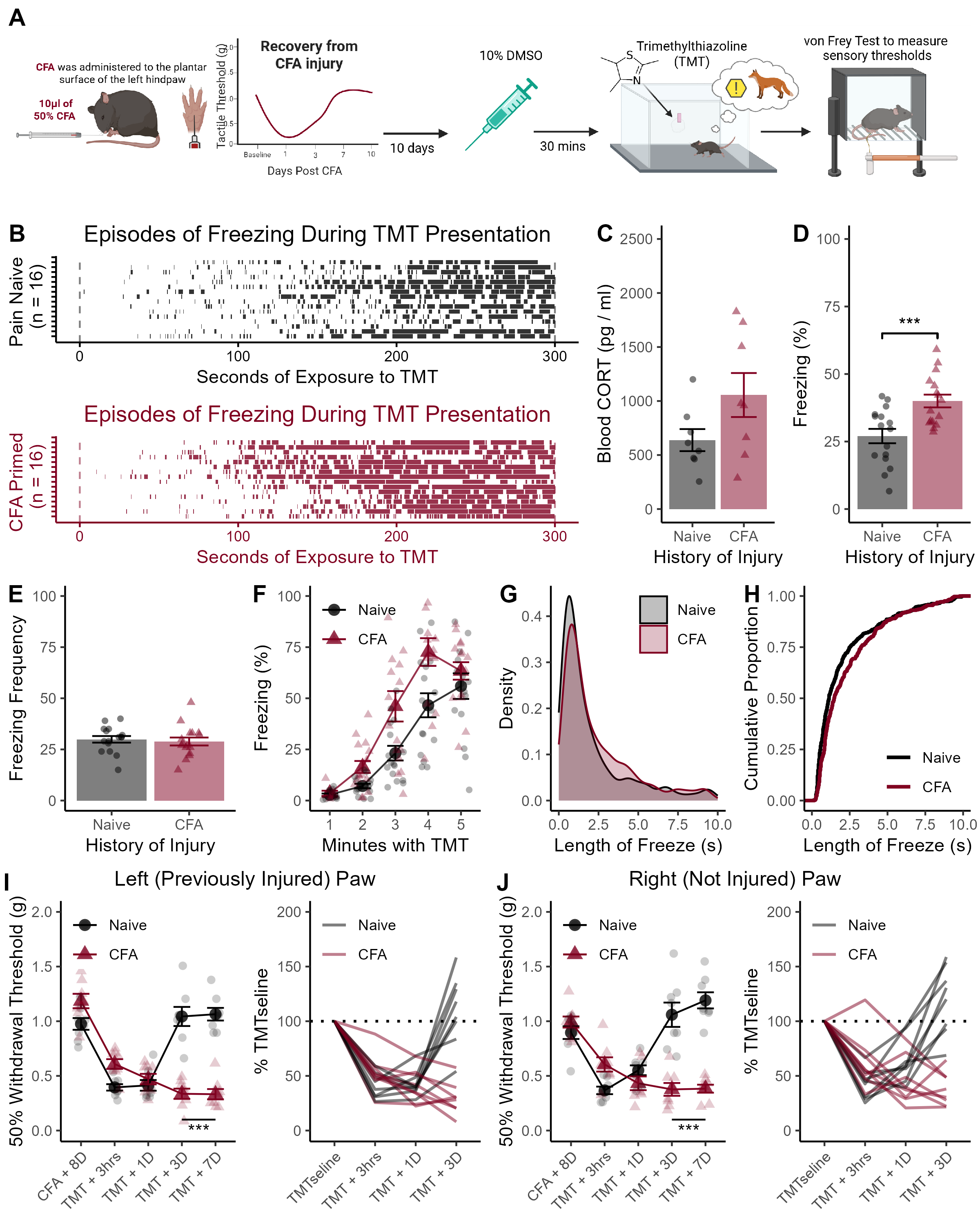
Supplemental Figure 5. Behavioral, hormonal and sensory responses to TMT after DMSO administration. (A) Timeline of experimental proceedings. Injury-naive controls and mice that had previously been injured with CFA and allowed to recover were administered 10% DMSO 30 minutes before exposure to TMT. (B) Raster plots of individual bouts of freezing during TMT exposure. (C) Blood levels of CORT 30 minutes after TMT. (D) Average time spent freezing during TMT. (E) Time spent freezing broken down by minute. (F) Number of freezing episodes during TMT. (G) Density plot of individual bouts of freezing during TMT. (H) Cumulative proportion of individual bouts of freezing across the session. (I) Mechanical hypersensitivity among mice with a history of CFA at the site of previous injury. (J) Expression of mechanical hypersensitivity was also expressed in the contralateral (no previously injured) hind paw for mice with a history of CFA. Data presented as mean value +/- SEM.
CORT Levels
##
##  Two Sample t-test
##
## data:  CORT by CFA
## t = -1.8313, df = 14, p-value = 0.08841
## alternative hypothesis: true difference in means between group Naive and group CFA is not equal to 0
## 95 percent confidence interval:
##  -905.95208   71.41745
## sample estimates:
## mean in group Naive   mean in group CFA
##            638.2211           1055.4884
The increased levels of blood-CORT among CFA-primed mice was not significant (p = 0.08).
Time Spent Freezing During TMT
b <- Exp_1_CFA.N  %>%
  filter(Behavior == "freeze") %>%
  group_by(ID,CFA) %>%
  summarise(
    sum=sum(Duration),
    Number=n(),
  ) %>%
  mutate(Perc = (sum / 300)*100) %>%
  mutate(Av_DUR = (sum / Number))
## `summarise()` has grouped output by 'ID'. You can override using the `.groups`
## argument.##
## Two Sample t-test
##
## data: Perc by CFA
## t = -3.6504, df = 30, p-value = 0.0009881
## alternative hypothesis: true difference in means between group Naive and group CFA is not equal to 0
## 95 percent confidence interval:
## -20.247317 -5.719725
## sample estimates:
## mean in group Naive mean in group CFA
## 27.02331 40.00683CFA-primed mice spent more time freezing that injury-naive controls (t30 = 3.65, p <0.001, figure S5D & E)
Frequency of Freezing During TMT
b <- Exp_1_CFA.N  %>%
  filter(Behavior == "freeze") %>%
  group_by(ID,CFA) %>%
  summarise(
    sum=sum(Duration),
    Number=n(),
  ) %>%
  mutate(Perc = (sum / 300)*100)
## `summarise()` has grouped output by 'ID'. You can override using the `.groups`
## argument.##
## Two Sample t-test
##
## data: Number by CFA
## t = 0.42099, df = 30, p-value = 0.6768
## alternative hypothesis: true difference in means between group Naive and group CFA is not equal to 0
## 95 percent confidence interval:
## -4.091773 6.216773
## sample estimates:
## mean in group Naive mean in group CFA
## 29.9375 28.8750There was no difference in freezing frequency (p = 0.67, Figure S5F).
Length of Freezing Bouts
a <- data %>%
  filter(Behavior == "freeze")

cfa_durations <- a$Duration[a$CFA == "CFA"]
naive_durations <- a$Duration[a$CFA == "Naive"]

library(kSamples)
ad.test(cfa_durations, naive_durations)
##
##
## Anderson-Darling k-sample test.
##
## Number of samples: 2
## Sample sizes: 462, 479
## Number of ties: 607
##
## Mean of Anderson-Darling Criterion: 1
## Standard deviation of Anderson-Darling Criterion: 0.75984
##
## T.AD = ( Anderson-Darling Criterion - mean)/sigma
##
## Null Hypothesis: All samples come from a common population.
##
## AD T.AD asympt. P-value
## version 1: 11.603 13.954 1.3197e-06
## version 2: 11.700 14.101 1.1609e-06The length of freezing episodes were longer for CFA-primed mice (D = 0.14, p < 0.001; Figure S5G, H). Relative to non-injured controls
Von Frey Sensitivity
## ANOVA Table (type II tests)
##
## $ANOVA
##     Effect DFn DFd      F        p p<.05   ges
## 1      CFA   1  14 28.452 1.05e-04     * 0.303
## 2     Test   4  56 41.981 3.08e-16     * 0.702
## 3 CFA:Test   4  56 39.826 9.13e-16     * 0.691
##
## $`Mauchly's Test for Sphericity`
##     Effect     W     p p<.05
## 1     Test 0.381 0.219
## 2 CFA:Test 0.381 0.219
##
## $`Sphericity Corrections`
##     Effect   GGe     DF[GG]    p[GG] p[GG]<.05   HFe     DF[HF]   p[HF]
## 1     Test 0.705 2.82, 39.5 4.51e-12         * 0.902 3.61, 50.5 7.5e-15
## 2 CFA:Test 0.705 2.82, 39.5 9.73e-12         * 0.902 3.61, 50.5 2.0e-14
##   p[HF]<.05
## 1         *
## 2 *## ANOVA Table (type II tests)
##
## $ANOVA
## Effect DFn DFd F p p<.05 ges
## 1 CFA 1 14 32.784 5.24e-05 * 0.368
## 2 Test 4 56 20.727 1.59e-10 * 0.527
## 3 CFA:Test 4 56 29.120 4.16e-13 * 0.610
##
## $`Mauchly's Test for Sphericity`
## Effect W p p<.05
## 1 Test 0.689 0.867
## 2 CFA:Test 0.689 0.867
##
## $`Sphericity Corrections`
## Effect GGe DF[GG] p[GG] p[GG]<.05 HFe DF[HF] p[HF]
## 1 Test 0.825 3.3, 46.21 4.88e-09 * 1.11 4.44, 62.17 1.59e-10
## 2 CFA:Test 0.825 3.3, 46.21 3.53e-11 * 1.11 4.44, 62.17 4.16e-13
## p[HF]<.05
## 1 *
## 2 *CFA-primed mice exhibited prolonged hypersensitivity in both the previously injured and the contralateral (not injured) hind paws after TMT exposure (Left Paw: F4,56 = 39.82, p < 0.001; Right Paw: F4,56 = 29.12, p < 0.001; Figure S5I & J, respectively)