Published Image
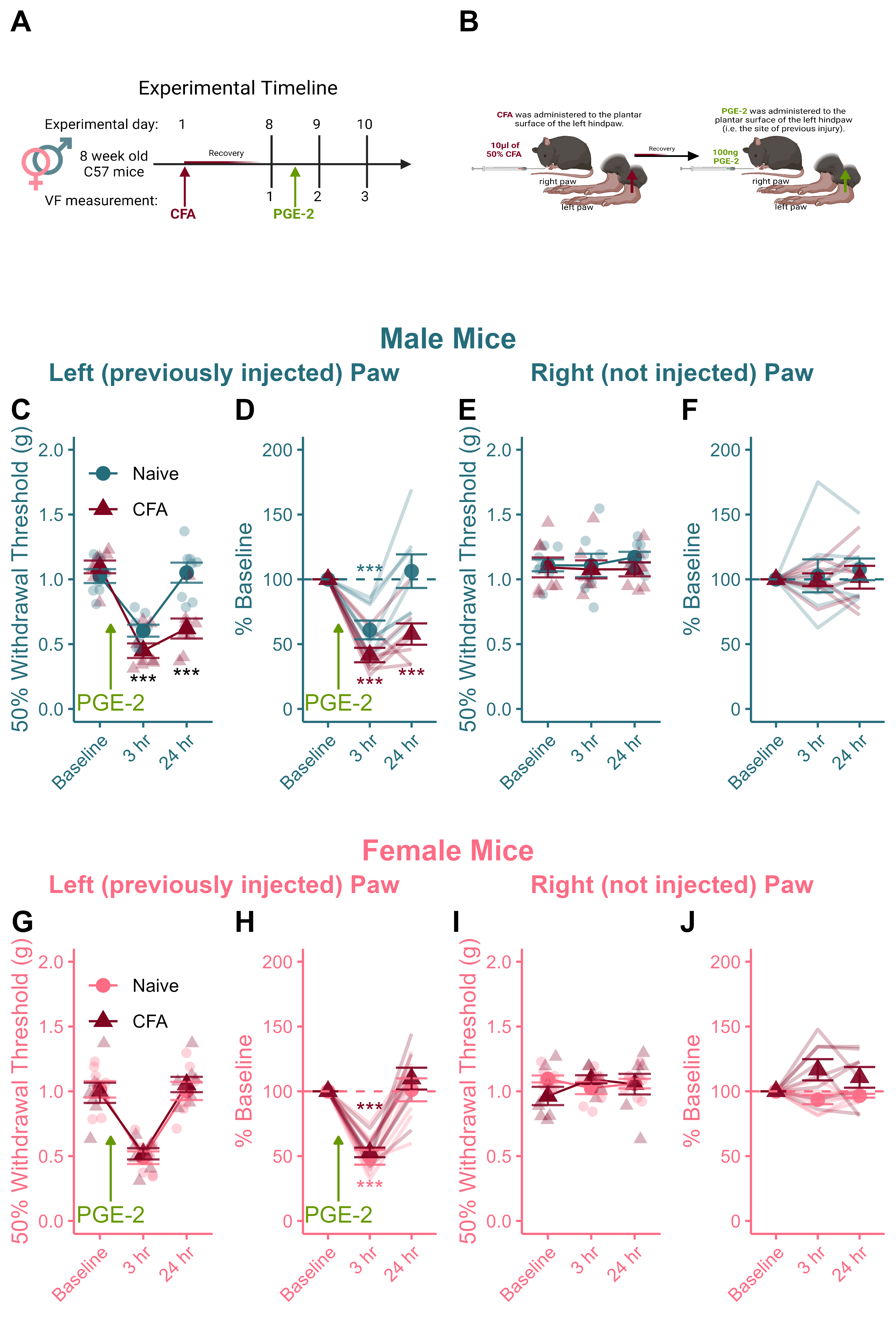
Figure 4. CFA-priming produced enhanced and prolonged mechanical sensitivity after PGE-2 injection in male mice only. (A) Timeline of experimental testing. (B) PGE-2 was administered to the site of previous injury to test expression of pain sensitization. CFA-primed male mice exhibited enhanced (3hr) and prolonged (24hr) mechanical sensitivity after PGE-2 injection relative to naive mice injected with PGE-2 (C). naive males recovered their baseline paw withdrawal thresholds 24 hours after PGE-2, whereas CFA-primed males exhibited ongoing sensitivity (C,D). There was no difference in the magnitude of mechanical sensitivity induced by PGE-2 injection 3hrs post administration in female mice (G), and both CFA-primed and pin-naive mice recovered basal levels of mechanical sensitivity 24 hours post-administration (H). There were no decreases in paw sensitivity in the contralateral (never-injected) paw during pain & recovery from PGE-2 administration (E,F,I,J). Data expressed as mean +/- SEM. \(***\) Indicates between-group difference where p < 0.001 and # indicates a within-subject difference from baseline where p <0.05.
Statistics
# Select the left paws
left_paws <- rbind(L_Male,L_Female)

# Remove those that did not receive PGE2 and switch to long form
a <- left_paws %>%
  filter(PGE2 == "PGE2") %>%
  melt(id.vars=c("ID","CFA","Sex","PGE2"))

# Run 3-way ANOVA: Sex X CFA X Day of testing (VF)
b <- anova_test(data=a,dv=value,between=c(Sex,CFA),within=variable,wid=ID)
knitr::kable(get_anova_table(b))
| Sex |
1 |
28 |
1.154 |
0.292 |
|
0.014 |
| CFA |
1 |
28 |
5.116 |
0.032 |
* |
0.060 |
| variable |
2 |
56 |
93.042 |
0.000 |
* |
0.684 |
| Sex:CFA |
1 |
28 |
7.754 |
0.010 |
* |
0.088 |
| Sex:variable |
2 |
56 |
5.705 |
0.006 |
* |
0.117 |
| CFA:variable |
2 |
56 |
3.548 |
0.035 |
* |
0.076 |
| Sex:CFA:variable |
2 |
56 |
6.479 |
0.003 |
* |
0.131 |
# Run both sets of follow ups:

## Effect of CFA on each day of testing split by sex
b <- a %>%
  group_by(Sex,variable) %>%
  pairwise_t_test(value~CFA)

tt(b)
| Sex |
variable |
.y. |
group1 |
group2 |
n1 |
n2 |
p |
p.signif |
p.adj |
p.adj.signif |
| Female |
Baseline |
value |
Naive |
CFA |
8 |
8 |
0.77900 |
ns |
0.77900 |
ns |
| Female |
3 hr |
value |
Naive |
CFA |
8 |
8 |
0.62900 |
ns |
0.62900 |
ns |
| Female |
24 hr |
value |
Naive |
CFA |
8 |
8 |
0.57000 |
ns |
0.57000 |
ns |
| Male |
Baseline |
value |
Naive |
CFA |
8 |
8 |
0.31600 |
ns |
0.31600 |
ns |
| Male |
3 hr |
value |
Naive |
CFA |
8 |
8 |
0.03960 |
* |
0.03960 |
* |
| Male |
24 hr |
value |
Naive |
CFA |
8 |
8 |
0.00087 |
*** |
0.00087 |
*** |
## Effect of Sex on each day of testing split by CFA history
c <- a %>%
  group_by(CFA,variable) %>%
  pairwise_t_test(value~Sex)

tt(c)
| CFA |
variable |
.y. |
group1 |
group2 |
n1 |
n2 |
p |
p.signif |
p.adj |
p.adj.signif |
| Naive |
Baseline |
value |
Female |
Male |
8 |
8 |
0.901000 |
ns |
0.901000 |
ns |
| Naive |
3 hr |
value |
Female |
Male |
8 |
8 |
0.086800 |
ns |
0.086800 |
ns |
| Naive |
24 hr |
value |
Female |
Male |
8 |
8 |
0.628000 |
ns |
0.628000 |
ns |
| CFA |
Baseline |
value |
Female |
Male |
8 |
8 |
0.232000 |
ns |
0.232000 |
ns |
| CFA |
3 hr |
value |
Female |
Male |
8 |
8 |
0.319000 |
ns |
0.319000 |
ns |
| CFA |
24 hr |
value |
Female |
Male |
8 |
8 |
0.000306 |
*** |
0.000306 |
*** |
## Effect of DAY within each group
d <- a %>%
  group_by(CFA,Sex) %>%
  pairwise_t_test(value~variable,p.adjust.method = "bonferroni")

tt(d)
| CFA |
Sex |
.y. |
group1 |
group2 |
n1 |
n2 |
p |
p.signif |
p.adj |
p.adj.signif |
| Naive |
Female |
value |
Baseline |
3 hr |
8 |
8 |
0.000002010 |
**** |
0.000006040 |
**** |
| Naive |
Female |
value |
Baseline |
24 hr |
8 |
8 |
0.879000000 |
ns |
1.000000000 |
ns |
| Naive |
Female |
value |
3 hr |
24 hr |
8 |
8 |
0.000002830 |
**** |
0.000008490 |
**** |
| Naive |
Male |
value |
Baseline |
3 hr |
8 |
8 |
0.000033200 |
**** |
0.000099500 |
**** |
| Naive |
Male |
value |
Baseline |
24 hr |
8 |
8 |
0.748000000 |
ns |
1.000000000 |
ns |
| Naive |
Male |
value |
3 hr |
24 hr |
8 |
8 |
0.000015600 |
**** |
0.000046700 |
**** |
| CFA |
Female |
value |
Baseline |
3 hr |
8 |
8 |
0.000010300 |
**** |
0.000030900 |
**** |
| CFA |
Female |
value |
Baseline |
24 hr |
8 |
8 |
0.441000000 |
ns |
1.000000000 |
ns |
| CFA |
Female |
value |
3 hr |
24 hr |
8 |
8 |
0.000001760 |
**** |
0.000005290 |
**** |
| CFA |
Male |
value |
Baseline |
3 hr |
8 |
8 |
0.000000103 |
**** |
0.000000308 |
**** |
| CFA |
Male |
value |
Baseline |
24 hr |
8 |
8 |
0.000009240 |
**** |
0.000027700 |
**** |
| CFA |
Male |
value |
3 hr |
24 hr |
8 |
8 |
0.049300000 |
* |
0.148000000 |
ns |