Supplemental Figure 1 - Sex Differences in Patterns of Homecage Behavior in Naive Mice
Published Image
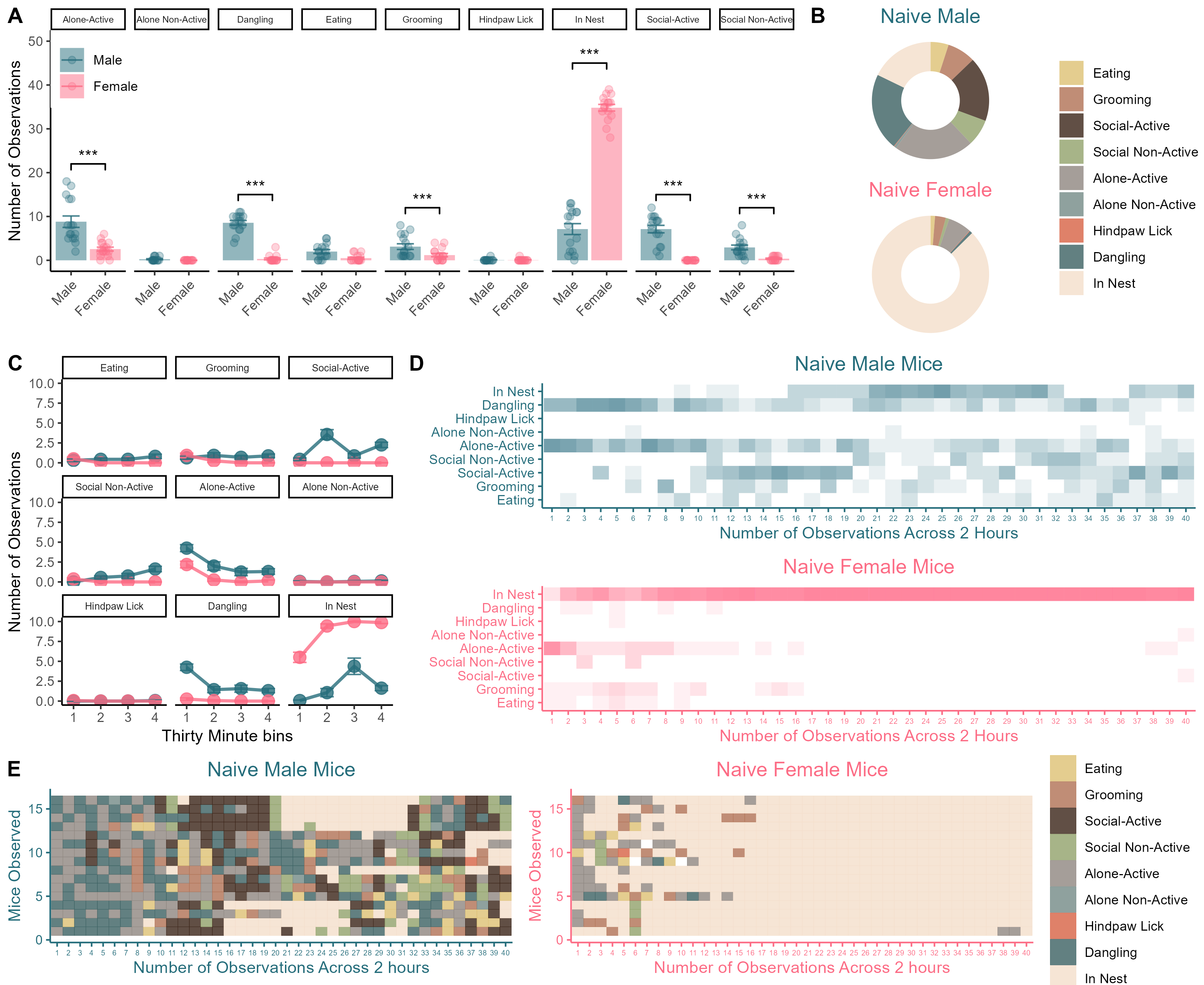
Figure S1. Sex differences in basal homecage behavior. (A) total quantification of observations across the two hour session expressed as mean value +/- SEM. (B) Donut charts showcasing the frequency of behaviors observed for males and females. (C) Line charts showing changes across the session divided into 4x30 minute bins. (D and E) are qualitative representations of the distribution of behaviors observed across the 40 timepoints.
Statistics
## MANOVA on SEX in the Naives:
a <- m_male_data %>%
  group_by(ID,Sex,value) %>%
  summarise(
    my_count=n()
  )

b <- dcast(a,ID+Sex~value,value.var = "my_count")

b <- b %>%
  mutate_at(c(3:12), ~replace(., is.na(.), 0))

fit <- manova(cbind(Grooming,`Social-Active`,`Social Non-Active`,`Alone-Active`,`Alone Non-Active`,`Hindpaw Lick`,`Dangling`,`In Nest`) ~ Sex, data=b)
summary(fit)
## Df Pillai approx F num Df den Df Pr(>F)
## Sex 1 0.974 107.69 8 23 0.0000000000000002247 ***
## Residuals 30
## ---
## Signif. codes: 0 '***' 0.001 '**' 0.01 '*' 0.05 '.' 0.1 ' ' 1# Because the omnibus test (above) is significant, follow up by running one-way ANOVAs for each behavior.
## Bonferroni correct these only if forced
summary.aov(fit)## Response Grooming :
## Df Sum Sq Mean Sq F value Pr(>F)
## Sex 1 30.031 30.0312 7.2547 0.01146 *
## Residuals 30 124.187 4.1396
## ---
## Signif. codes: 0 '***' 0.001 '**' 0.01 '*' 0.05 '.' 0.1 ' ' 1
##
## Response Social-Active :
## Df Sum Sq Mean Sq F value Pr(>F)
## Sex 1 406.13 406.13 74.405 0.000000001271 ***
## Residuals 30 163.75 5.46
## ---
## Signif. codes: 0 '***' 0.001 '**' 0.01 '*' 0.05 '.' 0.1 ' ' 1
##
## Response Social Non-Active :
## Df Sum Sq Mean Sq F value Pr(>F)
## Sex 1 52.531 52.531 22.944 0.00004214 ***
## Residuals 30 68.687 2.290
## ---
## Signif. codes: 0 '***' 0.001 '**' 0.01 '*' 0.05 '.' 0.1 ' ' 1
##
## Response Alone-Active :
## Df Sum Sq Mean Sq F value Pr(>F)
## Sex 1 312.50 312.500 21.988 0.00005597 ***
## Residuals 30 426.38 14.213
## ---
## Signif. codes: 0 '***' 0.001 '**' 0.01 '*' 0.05 '.' 0.1 ' ' 1
##
## Response Alone Non-Active :
## Df Sum Sq Mean Sq F value Pr(>F)
## Sex 1 0.5 0.5 5 0.03294 *
## Residuals 30 3.0 0.1
## ---
## Signif. codes: 0 '***' 0.001 '**' 0.01 '*' 0.05 '.' 0.1 ' ' 1
##
## Response Hindpaw Lick :
## Df Sum Sq Mean Sq F value Pr(>F)
## Sex 1 0.000 0.0000 0 1
## Residuals 30 1.875 0.0625
##
## Response Dangling :
## Df Sum Sq Mean Sq F value Pr(>F)
## Sex 1 544.50 544.50 228.86 0.000000000000001398 ***
## Residuals 30 71.38 2.38
## ---
## Signif. codes: 0 '***' 0.001 '**' 0.01 '*' 0.05 '.' 0.1 ' ' 1
##
## Response In Nest :
## Df Sum Sq Mean Sq F value Pr(>F)
## Sex 1 6132.8 6132.8 384.75 < 0.00000000000000022 ***
## Residuals 30 478.2 15.9
## ---
## Signif. codes: 0 '***' 0.001 '**' 0.01 '*' 0.05 '.' 0.1 ' ' 1- Females spent less time grooming (F(1,30) = 7.25, p = 0.01)
- Less socially active (F(1,30) = 74.405, p < 0.001)
- Less socially non-active (F(1,30) = 22.94, p < 0.001)
- Less alone active (F(1,30) = 21.988, p < 0.001)
- Less alone non-active (F(1,30) = 5, p = 0.032)
- Less dangling (F(1,30) = 228.86, p < 0.001)
… Because they spend so much more time than males in the nest (F(1,30) = 384.75, p < 0.001)